CS184/284A Spring 2025 Homework 3 Write-Up
Link to GitHub repository: https://github.com/cal-cs184-student/sp25-hw3-waffle
Overview
In this homework, we essentially implemented a mini ray tracer. We started out with generating camera rays that reduced aliasing and noise through Monte Carlo integration. From there, we worked on scene intersections, in particular ray triangle and ray sphere intersections. Then, to improve rendering efficiency, we constructed a bounding volume hierarchy (BVH). For the lighting phase of the project, we worked on both direct and global illumination. Finally, we finished off by integrating adaptive sampling into the renderer. This project took a lot of time, but it was extremely interesting to see just how drastic the effect of increasing the number of samples per pixel on reducing noise is on the final rendered picture. Additionally, due to the sheer amount of time this project took, it was extremely rewarding to see the final high quality rendered pictures! We learned a lot more about valuable insights into the trade-offs between quality and performance in ray tracing.Part 1: Ray Generation and Scene Intersection
Task 1: Generating Camera Rays
In the camera ray generation stage, the camera uses its own coordinate system. The camera is placed at the origin (0, 0, 0) and is oriented to look along the negative Z-axis. Given the camera’s field of view angles hFov and vFov , we define a virtual sensor plane located one unit away from the camera along the view direction (i.e., at z = -1). This sensor is defined so that its bottom left corner is at (−tan(hFov/2), −tan(vFov/2), -1) and its top right corner is at (tan(hFov/2), tan(vFov/2), -1).
After converting the passed in point into camera coordinates, it is then converted to world space with the transformation matrix c2w which becomes the direction of the ray.
Task 2: Generating Pixel Samples
For each pixel, multiple samples are generated . A random offset within the pixel (using a sampler) is added to the pixel’s bottom-left coordinates, then the result is normalized by the image width and height. Each sub-pixel sample produces a camera ray, which is traced through the scene. The radiance from all rays is accumulated and averaged to produce the final pixel color. This Monte Carlo integration reduces aliasing and noise in the rendered image.
Task 3: Ray-Triangle Intersection
I used the Möller–Trumbore algorithm. Given a triangle defined by vertices p1, p2, and p3, the algorithm proceeds as follows:
- Compute the edges: edge1 = p2 - p1 and edge2 = p3 - p1.
- Determinant calculation: the cross product of the ray direction and edge 2 is defined as a vector h, and the determinant of the dot product of edge1 and h is calculated to determine if the ray is parallel to the triangle
- Barycentric coordinates: if the ray is not parallel, the barycentric coordinates u and v are computed. The intersection point lies inside the triangle if u ≥ 0, v ≥ 0, and u + v ≤ 1.
- Ray parameter: The ray parameter t is calculated to determine the distance along the ray to the intersection. Only intersections with t within the ray's [min_t, max_t] range are considered valid.
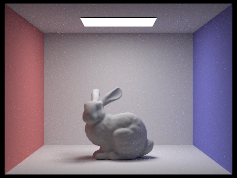
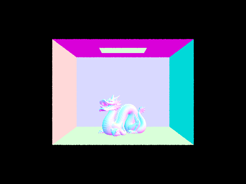
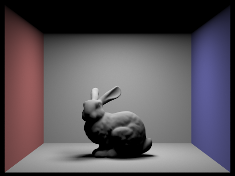
We then store this information inside the intersection structure. After these first three tasks, we were able to render the following:
Task 4: Ray-Sphere Intersection
The ray–sphere intersection is computed by solving the quadratic equation derived from substituting the ray equation r(t) = o + t·d into the sphere's equation (p - o)² = r². In our implementation, the sphere is defined by its center o and radius r (with r² precomputed). The quadratic coefficients are:
a = dot(r.d, r.d)
b = 2 · dot(r.o - o, r.d),
c = dot(r.o - o, r.o - o) - r².
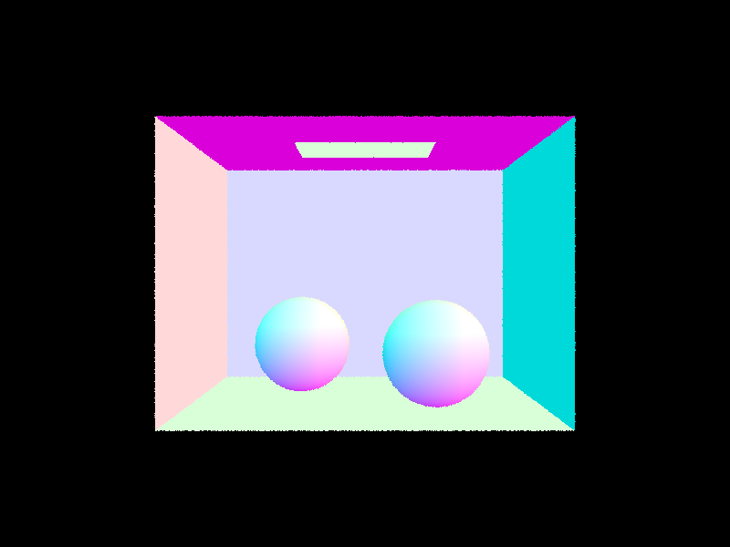
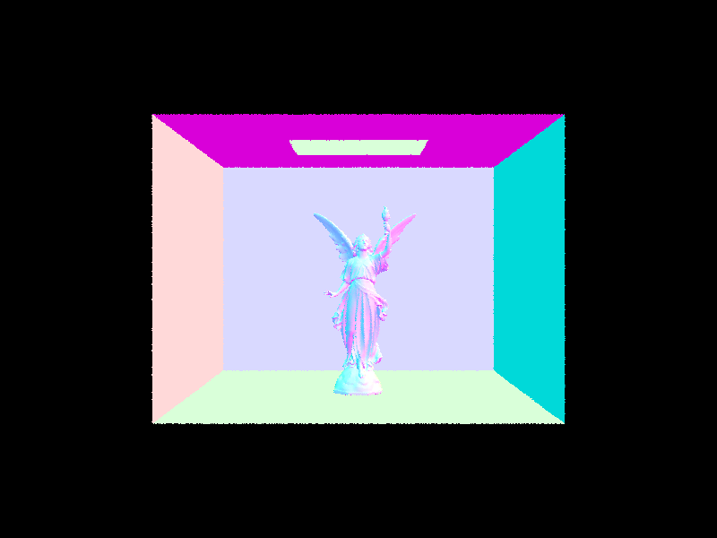
We then solve the quadratic equation to find t and check the validities of our solutions. Finally we update the intersection structure accordingly. This allows us to render the following output:
Part 2: Bounding Volume Hierarchy
The previous approach, while functional, takes a very long time to render especially as the number of primitives increase. This iis because we are performing a linear scan of all primitives for possible intersections which becomes expensive as scenes increase to thousands of primitive mesh elements. To adress this, we implement a bounding volume hierachy (BVH) — a data structure, similar to binary trees that wrap bounding volumes that form the leaf nodes of the tree.
Task 1: Constructing the BVH
To construct the BVH we start off by computing the bounding box of all
the primitives using Primitive::get_bbox() . We then
initalize a new BVHNode with that bounding box. If the number of
primitives is less than max_leaf_size , the node is a leaf
node, otherwise it is an internal node in which case we split the axis
by calculating the diagonal of the bounding box and comparing the x, y
and z components. The largest axis is chosen and split in half which
partitions the primitives. This function is recursively constructed on
the left and right subtrees.
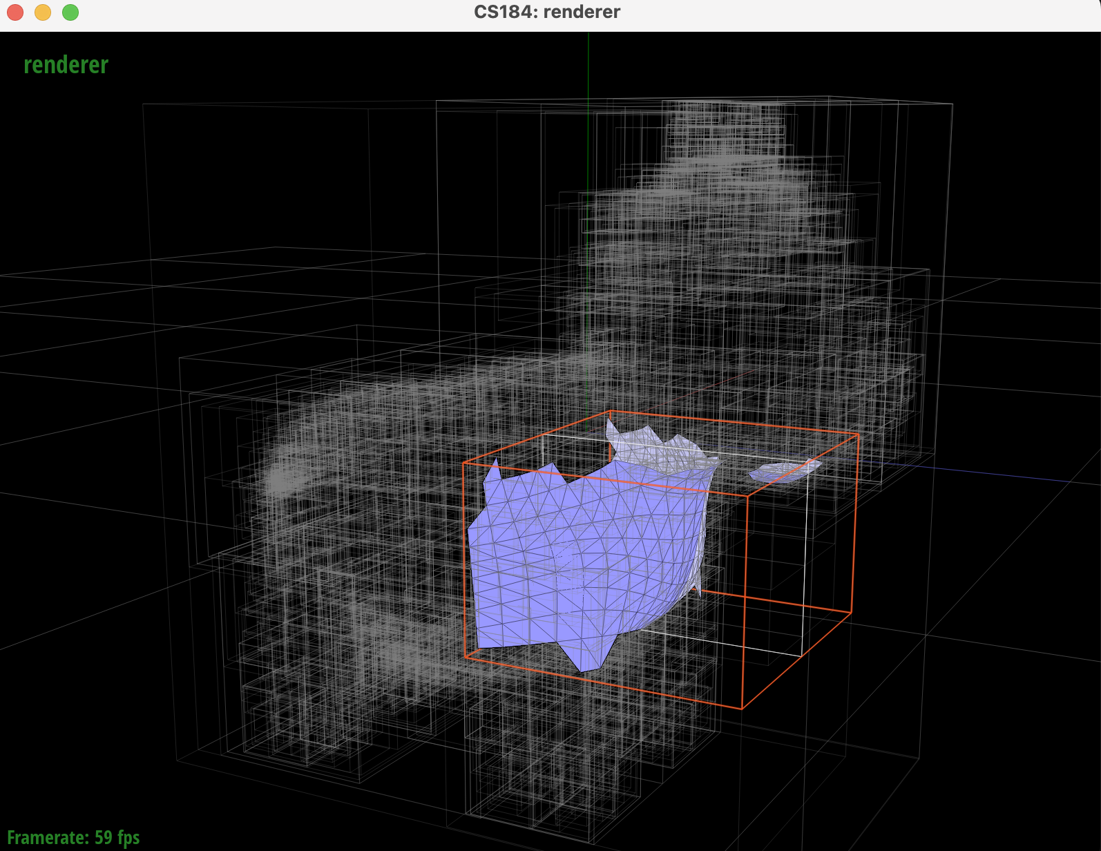
We can visualize the BVH using the GUI:
Task 2: Intersecting the Bounding Box
We also implement BBox::intersect() which takes a ray as
input and updates the input with the interval t values for
which the ray lies in the box. To implement this we use the ray and axis
aligned plane intersection equations from lecture:
t = (P′x − x) / dx
Where a ray is defined as P(t) = (x, y, z) + t · (dx, dy, dz) and an x-plane is defined by x = P′x.
In our implementation we compute the entry and exit t values for each axis and determine if the ray intersects the boudning box by calculating the overall entry and exit points. In the case the ray does intersect the bouding box, the algorithm recursively checks teh left and right children for leaf nodes and tests the ray against each primitive contained in the node.
Task 3: Intersecting the BVH
We now implement the intersection process for BVH. We start by doing a bounding box test to check if the ray intersects the node's bounding box. If its a leaf node we iterate over the primitives and test each for intersection, otherwise we will recursively traverse the left and right children give that the ray intersects the bounding box of the node. If either child reports an intersection the function can immediately return true, otherwise it can exit out. This allows us to discard nearly half of all primitives if the ray doesn't touch the bounding box.
After implementing BVHAccel::intersect() , we could
efficiently render files with thousands of primitives:

By comparing the average intersection tests per ray and render speed, we can see how much more efficiently the BVH accelerates rendering for various files/numer of primitives.
| Filename | Number of primitives | Rendering time (seconds) | Average speed (million rays/s) | Average intersection tests per ray | |||
|---|---|---|---|---|---|---|---|
| before | after | before | after | before | after | ||
| cow.dae | 5856 | 1.7403 | 0.0451 | 0.2640 | 3.7126 | 819.079338 | 5.700634 |
| CBlucy.dae | 133796 | 102.2147 | 0.0508 | 0.0016 | 2.7560 | 52615.023 | 6.677178 |
| wall-e.dae | 240326 | 262.7446 | 0.0458 | 0.0004 | 3.9004 | 133173.814 | 6.642789 |
The results show that a BVH can make a drastic improvement in rendering time by decreasing intersection complexity to logarithmic runtime. As expected with such runtime behaviour, the difference in rendering time is the greatest for wall-e which has the most number of primitives in comparison to cow.dae which has less primtives (and the rendering time difference is less drastic). With BVH, all of the files could be rendered in under a second!
Part 3: Direct Illumination
In this part we will start simulating light transport in the scene with realistic shading.
Task 1: Diffuse BSDF
Bidirectional Scattering Distribution Function (BSDF) is a generalization of the BRDF to represent materials that can both reflect and transmit light. BSDF objects itselves represent the ratio of incoming light scattered from incitent direction to outgoing direction.
We first support Lambertian surfaces, which are perfectly diffuse urfaces where reflect luinance is equal in all directions lying in the half space from the surface. As a result, the diffuse BSDF is constant and given by the equation:
\( f_r(\omega_i, \omega_r) = \frac{\rho}{\pi} \)
Where \(\rho\) is the surface reflectance/albedo ranging from total absorption to total reflection. This is divided by \(\pi\) to normalize the value.
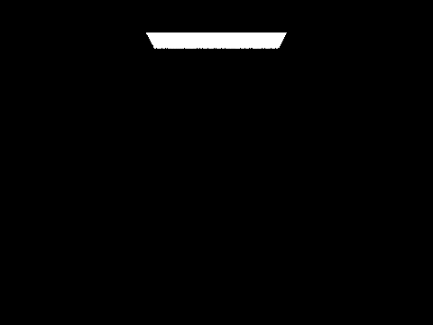
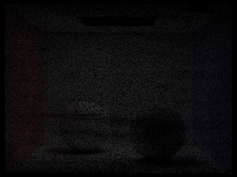
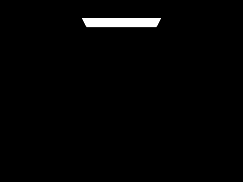
Task 2: Zero-bounce Illumination
Zero-bounce illumination refers to the light that reaches the camera directly from a light source, without any reflections, refractions, or bounces off other surfaces in the scene. In other words, it is the light that is emitted straight from an object (often an area light or an emissive surface) and travels directly to the camera.
This type of illumination is crucial for understanding the direct contribution of light sources in a scene. It forms the base level of the rendering equation by accounting for the light that doesn't interact with other surfaces before being captured by the camera. As a result, when we render a scene it shows the area light at the top of the box.
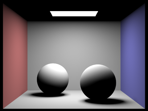
Task 3 + 4: Direct Lighting
For hemisphere direct sampling, we uniformly sample directions over the hemisphere using a dedicated sampler. Each sampled direction in the local space is transformed back into world space, before a new shadow ray is cast from the hit point in that direction. We add a small offset to avoid self intersections. If this shadow ray intersects an object, we retrieve the light's emitted radiance. Then, the BSDF at the hit point is evaluated for the outgoing and incident directions, weighted by the cosine of the angle between the sampled direction and the surface normal. We also normalize this number, by the PDF \( 1 / 2\pi \). All of these contributions are summed, and we divide by the number of samples to find an average, which is the estimate of direct lighting.
In contrast, importance sampling lights is a different form of direct sampling, where we target the light sources instead of uniformly sampling the hemisphere. We iterate over each light in the scene, and based on whether or not the light is a delta, the number of samples is either one, if it is a delta, or the size of the area light. For each sample, the function calls the light's own sampling routine to get the incident direction, the distance to the light, the emission of the light, as well as the pdf. The sampled light direction is then convered to local coordinates. A shadow ray is then cast towards the light source, with the maximum extent an epsilon short of the light's distance, to ensure that only the unobstructed light is considered. If the ray does not intersect anything, the BSDF for the incoming and outgoing directions is evaluated. The total contribution is the BSDF value multiplied by the light's emission and the cosine of the incident angle. This contribution is then normalized by dividing that contribution by the sample's PDF as well as the number of samples taken for that light. The final direct lighting value is obtained by summing up all of the contributions from all of the light samples.
|

|

|

|
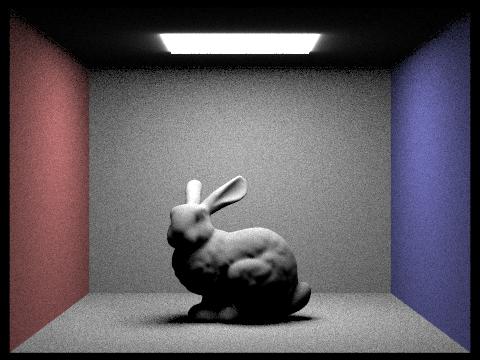
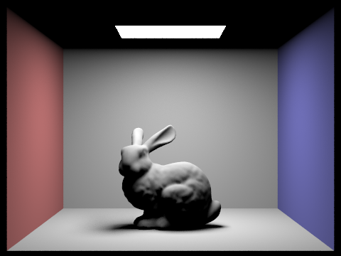
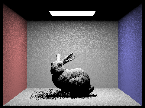
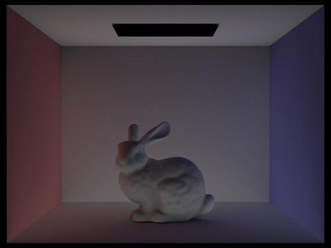
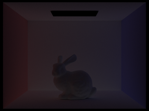
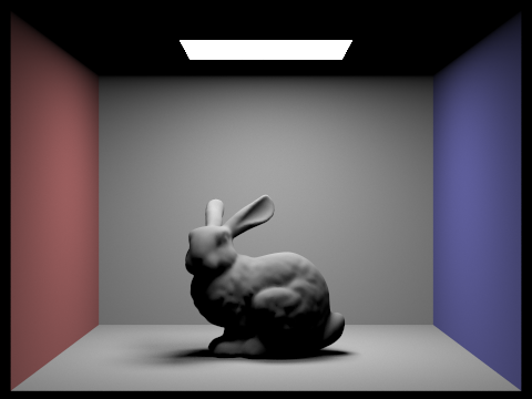
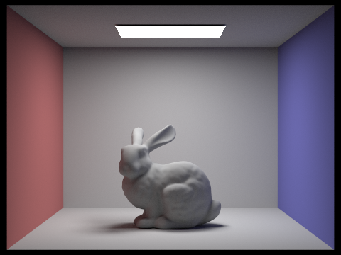
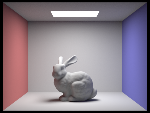
In these four pictures, as the number of light rays increases, the noise decreases in the soft shadows. In particular, the bunny's shadow becomes less harsh and more blended. With 1 light ray, the shadow is extremely pixelated and obvious. There are black dots scattered around. As the light rays increase, the shadow blends more, instead of black pixels, the shadow is scattered and diffused with varying shades of gray. In summary, increasing the number of light rays improves the quality and smoothness of soft shadows by reducing variance.
When I look at the difference between uniform hemisphere sampling versus light sampling, the most striking one is in the noise and clarity of the shadows. The bunny that was sampled uniformly, and uniform hemisphere sampling in general tends to have noisier results because it randomly samples all directions above the surface, many of which do not meaningfully contribute to the light from an area source. Thus, it takes more total samples to achieve the same level of smoothness in soft shadows. In contrast, light sampling focuses the sampling on the directions most likely to illuminate the point. As a result, for the same total number of samples, light sampling converges to cleaner shadows with significantly less noise. This is apparent in the two bunnies, where the one rendered with light sampling is much smoother, less noisy, and has less blur around the light source.
Part 4: Global Illumination
The indirect lighting function uses recursion. If
isAccumBounces
is true, the output radiance adds the one-bounce radiance. If it is
false, the output radiance is initialized to 0. If the ray's current
depth indicates that no further bounces are allowed, the base case is
reached and the function returns the one-bounce radiance. Else, the
function samples the BSDF to obtain a new direction, the pdf, and the
BSDF value. A 0 valued PDF immediately leads to returning the current
radiance. The new local direction is transformed into world space, and a
new ray is spawned (with a small offset) with its depth decreased. The
function tests whether this new ray intersects with anything. If an
intersection is found, it recursively calls itself to compute the
radiance contributed by subsequent bounes. This recursive component is
multiplied by the BSDF value and the cosine of the angle, and normalized
by the pdf. Depending on the accumulation setting, the contribution is
either added to the previously computed one-bounce radiance (if
accumulation is true), or replaces it (if accumulation is false). If no
radiance is detected and accumulation is false, the output radiance is
0. The function returns total radiance, which combines the direct and
recursive indirect contributions.
|
|

|
|
|
|
|

|
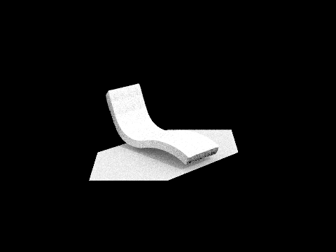
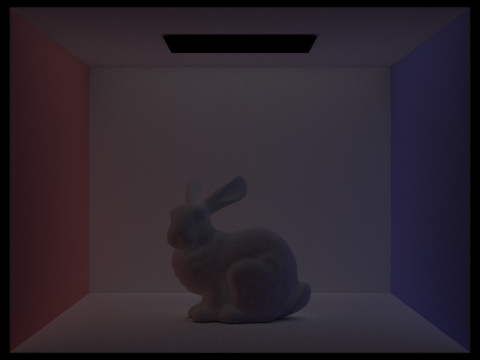
In the 2nd bounce of light, we can see that the light is coming from behind the bunny. This can be seen from the fact that the shadow is going to the front. In the 3rd bounce of light, the bunny itself changes and it is not as apparent that the light is coming from behind the bunny. Instead of the light sort of bending around the bunny, the bunny turns more one dimensional, since the shadows are not creating as much dimension. The quality of the image decreases as bounces of light increase. Rasterization tends to just make lines smoother. The non-accumulated recursive calls leads to an image getting darker and darker, more grainy, and lower quality.
|
|
|

|

|

|
The accumulated versions of the bunny are much brighter than the no accumulation versions. As the number of bounces increases, the no accumulation version gets progressively darker, and the accumulated versions get progressively brighter.
|

|
|

|

|

|
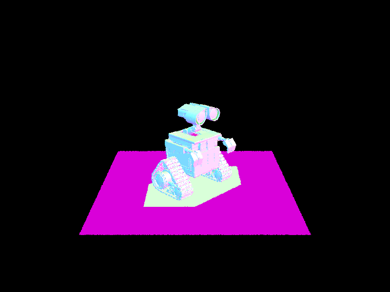
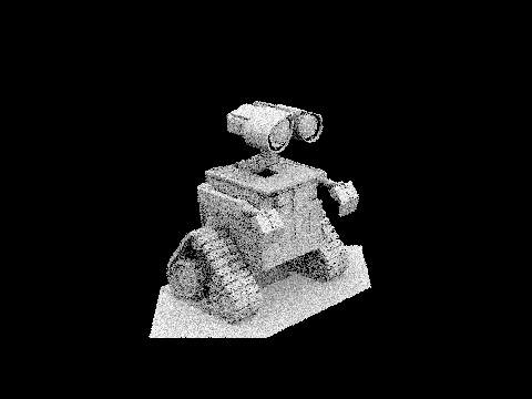
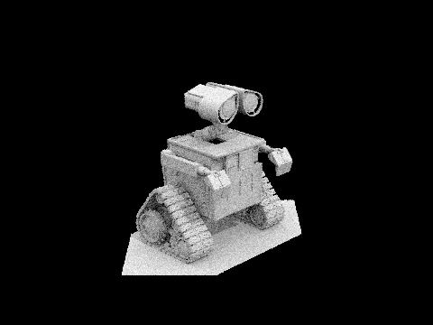
4 light rays used to render Wall-e
|

|
|

|

|

|

|
As the sample per pixel rate increases, the overall image quality increases. A sample per pixel rate of 1 leads to an extremely grainly looking Wall-E, with noticable black dots scattered throughout. A sample per pixel rate of 2 is also quite grainy, and the black specks are still apparent throughout. As sample per pixel rate keeps increasing, the black specks slowly start to disappear from Wall-E's body, and overall, the lines are much sharper and cleaner. At 1024 samples per pixel, all of Wall-E's lines are quite crisp, and there are not black specks scattered throughout his body, like with a sample per pixel rate of 1.
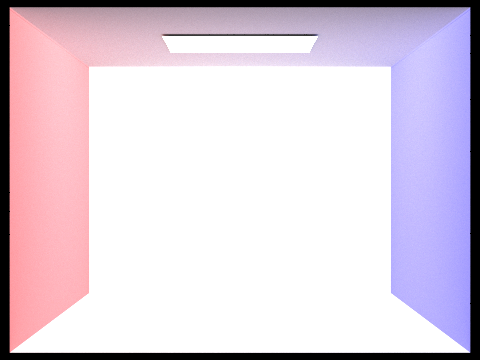
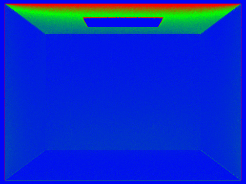
Part 5: Adaptive Sampling
In Monte Carlo path tracing, often times, a fixed number of samples per pixel is set to ensure that each pixel converges. However, not every part of an image needs the same number of samples. Some areas can converge quicker than others, and other parts converge slower. Adaptive sampling tackles this issue by monitoring the variance of the samples in each pixel and stops earlier for pixels that have already converged. This saves computation time by focusing more on samples on more difficult areas of the image.
I implemented it by first setting a maximum number of samples per pixel,
initializing the cumulative radiance and running totals regarding
illuminance. Keeping track of the number of samples taken thus far, the
main sampling loop is a while loop that continues until either the
maximum number of samples is acquired or the convergence criteria is
met. Within this while loop, a new batch of samples is acquired, up to
samplesPerBatch
per iteration. For each sample, we compute normalized pixel coordinates
and generates a camera ray with the appropriate depth setting. The
radiance for that ray is computed with the logic we implemented in
previous parts, and the resulting color is added to the total radiance.
We also keep track of running sums s1 and s2,
which keeps track of the samples illuminance and illuminance squared,
respectively. After each batch of samples, if at least 2 samples have
been collected, we calculate the mean illuminance and variance. Then, we
calculate I, a 95% confidence interval half-width. I is
then compared against a tolerance threshold multiplied by the mean
illuminance. If the condition that I is less than
maxTolerance * \(\mu\), the pixel's estimate has converged
and the loop will terminate early. The final color of the pixel is
determined by averaging the cumulative radiance over the number of
samples taken and this color is stored in the sample buffer. The actual
number of samples used is recorded in the sample count buffer.
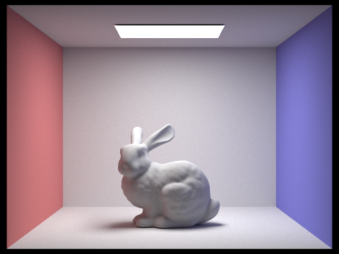
|
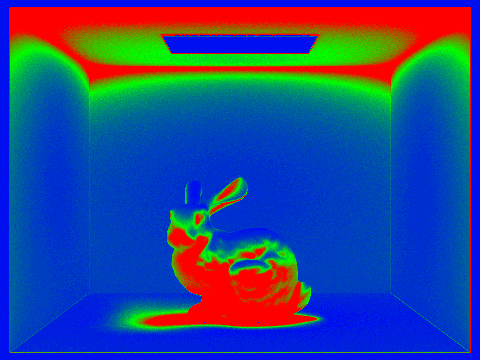
|
|
|